
Creative
Audio-reactive 3D particle systems in real time
How to build audio-reactive 3D particle systems: Euler physics, turbulent 3D noise force fields, spectral transient triggers, and GPU point rendering on a modular canvas.
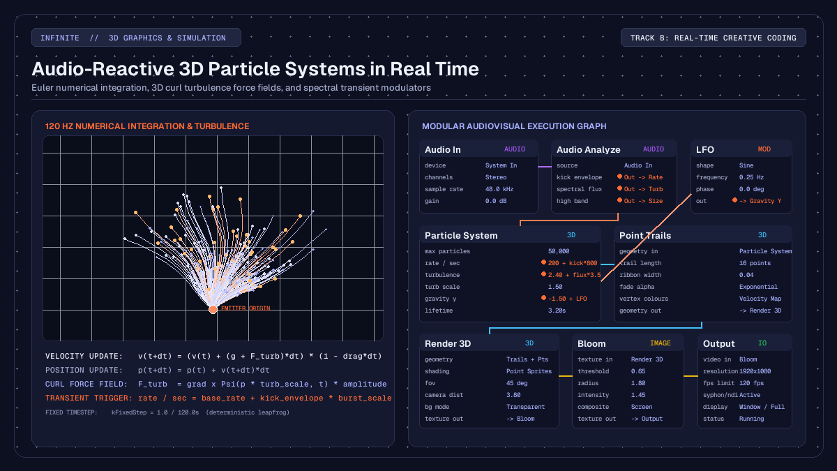
on this page
An audio reactive particle system transforms live musical transients and spectral frequencies into streams of kinetic points in three-dimensional space. From gentle dust motes drifting across an ambient soundscape to explosive shockwaves synchronised with sub-bass kick drums, particle systems provide an organic bridge between acoustic energy and computer graphics.
In real-time visual engines and audiovisual workstations like Infinite, audio and geometry share a unified execution graph. Rather than rendering pre-baked animations or relying on loose open sound control messages across network sockets, simulation nodes evaluate physical differential equations directly alongside audio-rate buffers. This enables deterministic, frame-accurate responses to rhythm and spectral timbre.
Here is how real-time particle mechanics operate under the hood, how numerical integration handles drag and velocity, how procedural 3D turbulence vector fields create fluid motion, and how to patch an audio-reactive particle pipeline using native nodes.

What makes particle systems feel musical
A common pitfall in generative music visualisation is mapping raw audio volume directly to particle count or size. When overall loudness drives everything, the visual output becomes a muddy, fluttering cloud that feels detached from the rhythmic structure of the music.
Musicality in a particle system requires separating three physical aspects of sound:
- Rhythmic transients: Sudden bursts of energy (such as kick drums, snare rimshots, and hi-hat attacks) should trigger discrete physical events: spawning a cluster of new particles or imparting an instantaneous impulse shockwave.
- Harmonic spectral balance: Sustained tonal components (such as basslines, synth pads, or vocals) should influence persistent environmental force fields: shaping gravity, drag, curl noise turbulence, and orbital attraction.
- Temporal decay and resonance: Particle lifetimes and trail lengths should correspond to musical tempo divisions, ensuring kinetic movement breathes in sync with the song rather than piling up into visual noise.
By decoupling instantaneous onset triggers from continuous vector fields, particles behave like physical matter reacting to sound waves propagating through a medium.
Numerical physics: fixed-step Euler integration
At the core of any particle engine is numerical integration: advancing position and velocity forward across discrete steps in time.
In Infinite, the Particle System node maintains an internal state array of particle records. Each particle stores position, velocity, remaining lifetime, initial lifetime, and scalar seed data.
To prevent simulation instability when frame rates vary during heavy rendering passes, the physics simulation runs on a fixed timestep:
kFixedStep = 1.0f / 120.0f; // 120 Hz internal physics updateIf a frame takes longer than usual (for example, during a window resize or shader compilation), the accumulator advances in discrete 120 Hz sub-steps up to a hard cap, preventing explosive time-step jumps.
The equations of motion
For each active particle at time t, the simulator computes acceleration by summing directional gravity g, external atmospheric forces, and fluid turbulence:
F_total = g + F_turbulence + F_externalThe updated velocity v(t + dt) applies acceleration and accounts for atmospheric drag:
v(t + dt) = (v(t) + F_total * dt) * (1.0 - drag * dt)Position p(t + dt) then advances along the newly computed velocity vector:
p(t + dt) = p(t) + v(t + dt) * dtLinear drag acts as a damping factor: without it, particles in an active turbulence field would continuously gain kinetic energy until flying off to infinity. Setting drag between 0.05 and 0.2 creates a natural terminal velocity reminiscent of smoke particles or underwater sediment.
3D turbulence and procedural vector force fields
Static directional gravity produces predictable fountain effects. To create organic, swirling motion where particles dance like embers or schooling fish, simulations apply procedural 3D noise vector fields.
Rather than sampling expensive perlin noise textures across memory, real-time particle kernels compute value noise and pseudo-curl fields analytically:
inline float Noise3D(float x, float y, float z)
{
    const float v = std::sin(x * 12.9898f + y * 78.233f + z * 37.719f) * 43758.5453f;
    return (v - std::floor(v)) * 2.0f - 1.0f;
}
In the Particle System node, turbulence is evaluated in three spatial dimensions:
float nx = Noise3D(p.x * turbScale, p.y * turbScale, p.z * turbScale + time);
float ny = Noise3D(p.x * turbScale + 19.1f, p.y * turbScale, p.z * turbScale);
float nz = Noise3D(p.x * turbScale, p.y * turbScale + 31.7f, p.z * turbScale);

F_turbulence = Vec3(nx, ny, nz) * turbulenceAmount;
When turbulence is modulated by an audio feature (such as spectral flux or mid-frequency energy), complex vortex structures suddenly twist and expand whenever an instrument enters the mix, returning to laminar flow during quiet breakdowns.
Isolating audio transients for explosive particle bursts
To create tight rhythmic synchronisation, incoming audio must pass through envelope extraction before reaching the particle emitter.
In a modular graph, the Audio In node captures multi-channel audio from your interface, system sound, or DAW routing. This feeds directly into an Audio Analyze node, which divides the audio spectrum into frequency bands and tracks both peak amplitudes and transient envelopes:
- Sub-bass band (20 Hz to 120 Hz): Isolates kick drums and bass stabs. Connecting this output to the particle emitter's
rate / secparameter creates explosive bursts on downbeats. - Spectral flux: Measures the rate of change across frequency bins. A sudden brass chord or snare strike produces a high spectral flux value, ideal for driving
turbulenceorspread. - High-frequency envelope (6 kHz to 16 kHz): Tracks hi-hats, shakers, and cymbal sizzle. Modulating particle
start sizeorspeed randomwith high frequencies adds crisp kinetic shimmer to rapid rhythmic passages.
Because modulation values update at UI and block intervals without latency, particle emission synchronises tightly with what the audience hears.
Point trails, ribbon geometry, and GPU rendering
Individual floating points can look sparse on large display projections. To give particles visual weight and continuity, Infinite pairs the Particle System with downstream geometry generators and compositing nodes.
Turning points into continuous ribbons with Point Trails
The Point Trails node samples point positions across successive frames and extrudes them into continuous triangle strips. As particles whip through turbulent vortices, their trajectories form luminous ribbons through space.
Key controls in Point Trails include:
trail length: Determines the historical sample depth (from 4 to 64 steps). Shorter trails produce comet tails; longer trails create intricate calligraphic ribbons.ribbon width: Defines the cross-sectional geometry size in world space.fade alpha: Tapers opacity exponentially towards the tail so older segments dissolve smoothly into the background.
Point sprite rendering in Render 3D
Both raw particles and ribbon meshes connect directly into the Render 3D node. For dense point clouds containing tens of thousands of elements, Render 3D uses hardware-accelerated point sprites. Rather than drawing individual quad polygons, a single vertex shader call computes screen-space point sizes while fragment shaders evaluate circular alpha falloffs and depth fading.
Adding a Bloom node downstream extracts specular highlights from high-density particle clusters, wrapping them in a natural optical glow. A subtle Color Adjustments pass allows fine-tuning contrast and grading the colour palette to match the mood of the performance.
You can also explore how audio-reactive shaders compare to geometric pipelines in our guide to audio-reactive GLSL shaders.
Complete example patch
Here is a complete, reproducible Infinite patch demonstrating an audio-reactive 3D particle system. It sets up an audio input, transient analysis, a high-capacity particle generator, point trails, a 3D camera renderer, optical bloom, and screen output.
You can paste this plain text directly into an .inf file or inspect it to understand the node connections:
infinite-patch 1
rev 2
# Audio-Reactive 3D Particle System: transient bursts, curl turbulence, and bloom

node 1 Audio Audio In
  id audio_in
  pos 120 280
end

node 2 Audio Audio Analyze
  id analyze
  pos 380 280
end

node 3 Modulator LFO
  id lfo_sway
  pos 380 460
  param shape 0
  param frequency 0.15
end

node 4 3D Particle System
  id particles
  pos 700 280
  param max_particles 30000
  param rate 180
  param shape 1
  param radius 0.25
  param lifetime 3.5
  param speed 1.8
  param spread 0.45
  param dir_y 1.0
  param gravity_y -1.2
  param drag 0.12
  param turbulence 2.2
  param turb_scale 1.4
  param start_size 0.05
  param end_size 0.01
end

node 5 3D Point Trails
  id trails
  pos 1020 280
  param length 18
  param width 0.03
  param fade 0.85
end

node 6 3D Render 3D
  id renderer
  pos 1320 280
  param fov 45.0
  param cam_dist 4.2
  param shading 1
end

node 7 Image Bloom
  id bloom_fx
  pos 1600 280
  param threshold 0.60
  param radius 2.0
  param intensity 1.4
end

node 8 Image Color Adjustments
  id color_grade
  pos 1860 280
  param contrast 1.15
  param saturation 1.25
end

node 9 Utility Output
  id out_screen
  pos 2120 280
end

# Wiring
cable analyze 0 audio_in 0
cable particles 1 analyze 1        # Kick transient envelope -> Particle Emit Rate
cable particles 11 analyze 2       # Spectral flux -> Turbulence intensity
cable particles 9 lfo_sway 0       # Slow LFO -> Gravity Y drift
geo trails 0 particles
geo renderer 0 trails
cable bloom_fx 0 renderer 0
cable color_grade 0 bloom_fx 0
cable out_screen 0 color_grade 0
When live audio plays through Audio In, kick transients trigger dense bursts of new points while spectral changes continuously alter the curl turbulence, causing the trails to swirl in synchrony with the music.
Performance and buffer limits
Running tens of thousands of particles in real time alongside audio DSP requires keeping CPU and GPU overhead predictable:
- Particle capacity: On modern hardware,
Particle Systemcomfortably simulates 20,000 to 50,000 particles at 120 frames per second. If your project targets portable laptops or high-resolution multi-projector setups, keepingmax particlesbetween 15,000 and 25,000 ensures plenty of GPU headroom for post-processing shaders. - Lifetimes and garbage collection: Shorter particle lifetimes (between 2.0 and 4.0 seconds) cycle dead particles out of the buffer quickly, preventing memory bloat during prolonged high-tempo sections.
- Trails depth:
Point Trailscreates geometric triangle meshes for each particle. If particle counts exceed 30,000, consider reducinglengthto 8 or 12 points to minimise vertex memory bandwidth.
For ready-to-run templates, generative synths, and community visual rigs, visit the Infinite library. You can download Infinite for macOS, Windows, and Linux from the download page and begin patching generative audiovisual instruments immediately.